Gain more self-assurance analyzing visual outputs in IKOSA by learning how to interpret confidence maps for semantic and instance segmentation.
| Note |
|---|
Important: confidence map visualizations are relevant only for semantic and instance segmentationtraining types! |
While looking at the results outputs of a trained model in IKOSA you will often be confronted with different visual representations. One such type of visualization is the ‘confidence map.’ In order to make sense of your visual outputs, you have to be familiar with the purpose of confidence maps.
In this article, we introduce you to the concept of confidence maps and provide instructions on how to read the different confidence levels displayed in the representations.
What to expect from this page?
| Table of Contents | ||||||
|---|---|---|---|---|---|---|
|
📑 What is a confidence map?
The confidence map is the actual visual output of semantic and instance segmentation jobs in IKOSA. A confidence map is a visualization produced for each class (label) in the output of a trained application. It displays a value lying between 0 and 1 which is assigned to each pixel of the original input image. This value denotes the probability of a pixel belonging to a certain class (label).
To yield the segmentation map, which later serves as the basis for analysis results and for calculating the app’s performance, a 'confidence threshold' is applied.This threshold is the baseline against which you can determine whether a certain pixel belongs to a given class or not.
The confidence threshold is set to 0.5 in all IKOSA applications. Thus, a pixel with a confidence level lower than 0.5 will be regarded as “not belonging to a certain class,” while pixels with confidence levels higher than 0.5 will be regarded as “belonging to a certain class.“ The relative distance from the threshold does not play a role when assigning pixels on the same side of the spectrum to a particular label. Thus, a pixel with a value of 0.051 will be equally regarded as belonging to a given label just as a pixel with a value of 0.99.
📑 Interpreting confidence maps
Confidence map visualizations provided as an output in IKOSA consists of two sections:
(1) Input image
(2) Confidence map
| Info |
|---|
Please note: confidence map visualizations are downscaled to 25 megapixels (MP), if the original image size is larger than 25 MP. |
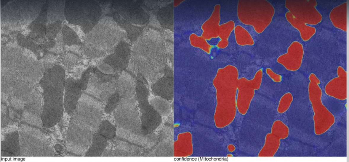
Input image (Left image)
This visualization displays the original input image.
Confidence [your-label-name] (Right image)
This visualization displays an overlay of a trained model’s confidence values for a given label on top of the input image.
Each colors on the colormap below corresponds to the confidence level for a certain region on the image. Confidence levels range from dark blue (very low values) to bright red (very high values).

The confidence threshold value of 0.5 is marked green in the color bar above. Values on the left side of the bar, marked with different shades of blue, are regarded as not belonging tothe given class (label). On the other hand, values on the right side of the bar, marked with a shade of yellow or red, are regarded as belonging to the given class (label).
You’ve made great progress by adding confidence map interpretation to your image analysis skills. Now you are equipped to gain deeper insights into your visual outputs!
Help a colleague interpret the visual outputs of their analysis!
If you still have questions regarding your application training, feel free to send us an email at support@ikosa.ai. Copy-paste your training ID in the subject line of your email.
📚 Related articles
| Filter by label (Content by label) | ||||||||||
|---|---|---|---|---|---|---|---|---|---|---|
|